On removing abnormal claims from reserving triangles

The main idea: iteratively replacing the highest deviating cell in a reserving triangle with the expected result for that cell removes without ignoring abnormally large claims. 

0. Posts on this blog are ranked in decreasing order of likeability to myself. This entry was originally posted on 27.10.2021, and the current version may have been updated several times from its original form.

 

1.1 In a previous post I discussed a general method for removing outliers from a dataset given that one has a model. Let's try now to apply this to non-life claims reserving by triangles.

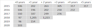
1.2 The cumulated triangle below includes one obvious outlier incurred in 2018, and emerging one year after.

1.3 Having a model of the data arranged in triangle form means breaking down the triangle into a vertical (exposure) and horizontal (pattern) component. These two are dependent on the choice of reserving method, with the additive method being an obvious example of splitting the triangle into two dimensions.

1.4 Let’s work with basic chain ladder instead. Now we could use year 0 claims as a measure of exposure and the cumulated development factors as a pattern, but this would mean that we always “take for granted” that year zero data.

1.5 A better approach is to use the ultimate development as exposure. You can go about calculating the ultimate by the usual longish fashion, or you can use a shortcut as below, where you go by iteration calculating the ultimate development of the earlier to the latter years, with the ultimate development of the earliest year just being that year’s final datapoint (assume tails away).

1.6 The next ultimate then is, if we stick to the color scheme below, BLUE = YELLOW x SUM OF GREEN / SUM OF ORANGE. Iterative procedure but will give you the ultimates rather quicker than going through the dev factors drama.

1.7 Next we use the ultimates (our measure of exposure) to derive the pattern, which is just the sum of cumulated development at each interval divided by the sum of exposure, in like fashion to the additive method. If you really miss your development factors, you can derive them easily from the pattern by dividing successive terms (or all terms by the first one if you need cumulative factors).

1.8 Now we have the model of the triangle, and we can create a “synthetic” triangle by multiplying exposure and pattern.

1.9 Next, we calculate the absolute difference between the actual and synthetic triangles, and isolate the greatest such difference.  In this case, this will be a difference of $ 202 between the synthetic value of $ 299 and the real value of $97 in the first development year of 2018.

1.10 Now Replace the 97 in the original triangle with the 299 in the synthetic and re-run all calcs. By all I mean all, exposure, pattern, synthetic triangle, differences, replace the sore thumb.

1.11 repeat until the greatest difference between the two triangles is arbitrarily small. You get this

1.12 Notice how the procedure has not changed the leading edge of the triangle, i.e. does not change the amount of development experienced (if you use a cumulative triangle, which you should).

1.13 What has changed is when this development appears, which is obvious if you look at the difference in development pattern, where the obvious outlier in the original triangle was making it look as if only 21% of the total development was done by year zero (smoothed figure closer to 40%). 40% of development in year zero is close to the 38% average of all years except the 2018 outlier.

1.14 What I really like about this application is that it gives me a way to use the full claims history without having to make a judgement call on what to consider big or abnormal claims. Chuck it all in there, God will recognize his own.