On removing outliers

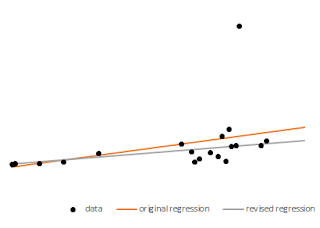
The main idea: iteratively replacing the datapoint most distant from the expected by the latter allows a model to account for outliers without ignoring them.   

0. Posts on this blog are ranked in decreasing order of likeability to myself. This entry was originally posted on 17.10.2021, and the current version may have been updated several times from its original form.

1.1 Another technique which would be rather obvious, just writing about it as I don’t remember encountering it. The application to claims reserving could be a bit more original, that’s coming in a next post.

1.2 So, a technique that would help to smooth out any outliers in your dataset (as long as you have a model of the underlying pattern, which if you don’t, how do you know that you even have outliers?) is to iteratively replace the datum that diverges by most (absolute value or percentage, depending on context) by the expected datum by the latter. Recalculate the model parameters given the new data, and repeat until there are no more outliers form the model at all (arbitrary small differences).  There, you have model parameters that are robust against outliers.

1.3 Alternatively, you can replace the offending datum by a weighted sum of the datum and its expected value, which will allow the smoothing process to take a bit longer.

1.4 In all cases, you are not ignoring outliers, as these are “baked in” the model parameters that you use to generate the expected value you replace the outlier with. You are just lessening their influence.

1.5 Example below, data point I have created by applying a Y = 1 + X model but building some random variation around that, as well as manually increasing one datum to be the obvious outlier. Apparent intercept is of 0.8661 (true intercept of 1) and apparent slope is of 1.5766 (true slope of 1).

1.6 Now I apply the steps above by macro, and I end up with the following smoothed parameters, apparent intercept is of 0.9986 (true intercept of 1) and apparent slope is of 0.9137 (true slope of 1). Better eh?

1.7 I repeated this but now I replaced the offending datum with a weighted sum of 99% datum and 1% model, and I get an apparent intercept is of 0.9926 (true intercept of 1) and apparent slope is of 0.9405 (true slope of 1). One better the other worse, so not obvious that the good two minutes the macro took to run this one were a wise investment.

1.8 Now, in the example above I only replaced the Y values, but in reality you would run a function predicting Y from X, and another predicting X from Y, and run the algorithm on both independently of one another. 

1.9 "Independently" except that the replaced Y would inform the X function, and the replaced C would inform the Y function as soon as the replacements are made.

1.10 What this does is that it finally gives you two regressions that are compatible: the intercept and slope of one are transmuted into the other. Show me where else you can get this. No, no, show me.

1.101 An alternative use of this algorithm is in dimensions reduction. Let's say you have separated the factors you want to reduce to two into as many bundles, one of which has N such factors. You run N multiple regressions whereby you predict each factor from the others in turn, and then run the above.

1.102 Note that you have to make the models mutually consistent, and when you replace a datum in each was per above, you replace that same datum in the N-1 other models (as an independent variable). So, at each turn you replace 1 datum in each of the N factors and N^2 data in the N models.

1.103 Once you are done and no errors remain whatsoever, you'll have reduced all the N factors into the same linear uber-factor. And thus, have reduced dimensions for those N factors.